
")
The financial markets constitute a socioeconomic ecosystem where individuals, organizations and institutions can trade various financial instruments (metals, currencies, stocks, securities, indices, oil, and now cryptocurrencies, etc.). Here these instruments are traded at a fair cost and on the basis of demand and supply. Trading the financial markets carries a substantial amount of risk and the need to make adequately informed decisions (while trading) cannot be overemphasized. While concepts like Technical analysis (via price action) and fundamental analysis are reasonably effective, it is imperative to have a solid trading plan and strategy that is robust and sustainable.
Personally, I do not believe that any financial instrument completely exhibits Brownian behavior. This is because prices will usually respect key historical zones (supply and demand zones) as well as market channels. A good example can be seen in the volatility 10 index chart below (the demand zone is marked with green lines and the supply zone is marked with red lines, the market channel was is also marked with a red diagonal trend line).
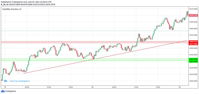
From the chart we can see that the price occasionally bounced-off the marked zones and this forms the basis for price-action trading.
Register for Tekedia Mini-MBA edition 18 (Sep 15 – Dec 6, 2025) today for early bird discounts. Do annual for access to Blucera.com.
Tekedia AI in Business Masterclass opens registrations.
Join Tekedia Capital Syndicate and co-invest in great global startups.
Register for Tekedia AI Lab: From Technical Design to Deployment.
Some statistical tests can be carried out on the close price of financial instruments (to ascertain key metrics which can further be used to better understand market behavior); one of which is the Augmented Dickey-Fuller test. This test is used to check if a particular asset or instrument will revert to its rolling mean after a market swing (in upwards or downwards direction).
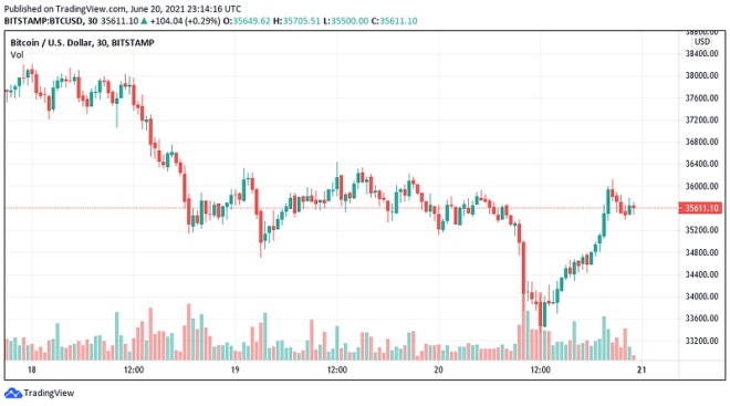
The Bitcoin stock-to-flow model makes it possible to trade it against a base currency on the foreign exchange market. This means that as with the Volatility 10 index above, bitcoin can be represented (on the charts) by its open, high, low and close prices and consequently traded with leverage at varying trade volumes. The bitcoin chart can be seen below.
Seeing that there exists a degree of repetitive behavior of in price movement, can this behavioral pattern be recognized by a machine learning model?, if yes what model could be ideal?

Well, I hope that this article guides your discretion in answering these questions. For demonstration I have used the bitcoin price data (from April 2013 to February 2021) as obtained from kaggle.
WHY LSTM?
LSTM (Long Short-Term Memory) is a deep learning model that helps with prediction of sequential data. LSTM models prevail significantly where there is a need to make predictions on a sequence of data. The daily OHLC (Open, High, Low and Close) price of any financial asset constitutes a good example of a sequential data.

IMPLEMENTATION
As proof-of-concept, I have implemented an LSTM model for predicting Bitcoin’s price using python. I have outlined my step-by-step procedure as well as my thought process every step of the way. Without further ado, let’s go!
Firstly, we import the requisite python libraries
import numpy as np #Python library responsible for numerical operations
import pandas as pd # The pandas dataframe is a python data structure that helps construct rows and columns for data sets`
import matplotlib.pyplot as plt # This library is responsible for creating the necessary plots and graphs
import tensorflow # This is a python framework with which different models can be easily implemented
INGESTING THE DATA SET
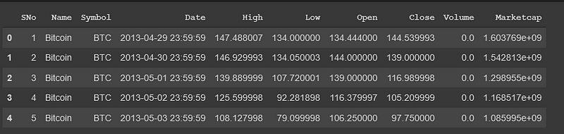
data = pd.read_csv(‘coin_Bitcoin.csv’) # Here we are simply using pandas to import the csv file containing the BTC data
data.head() # Taking a quick look at the first 5 rows of the data
We only require the Date, High, Low, Open and Close columns and so we drop every other column. Since it is a time-series data, it is best to set the date column as index. This way we can easily observe price behavior over time.
required_data = data[[‘Date’,’High’,’Low’,’Open’,’Close’]]
required_data.set_index(“Date”,drop=True,inplace=True)
required_data.head()
Now the dataset looks like this:
In a bid to ascertain more insights on price changes, we create a column that constitutes the daily Logarithmic returns. The reason we are interested in this metric is partly because stock returns are assumed to follow a log normal distribution and also because log returns is a more stationary property than the regular arithmetic returns.
Thus,
required_data[‘% Returns’] = required_data.Close.pct_change() # we find the percentage change using the pct_change() method
required_data[‘Log returns’] = np.log(1 + required_data[‘% Returns’]) # from the percentage returns we can easily compute log returns
required_data.dropna(inplace=True) # We drop all null/NaN values so that we do not get a value error
I have used the close price and log returns in training the model inputs because the close price is usually the most effective parameter for evaluating price changes, and the log returns offers stationarity to the model.
Let’s take a look at the close price curve:
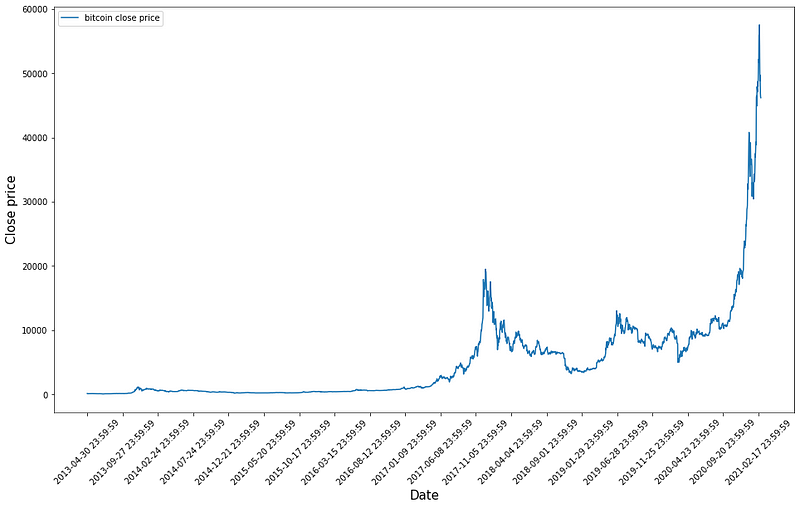
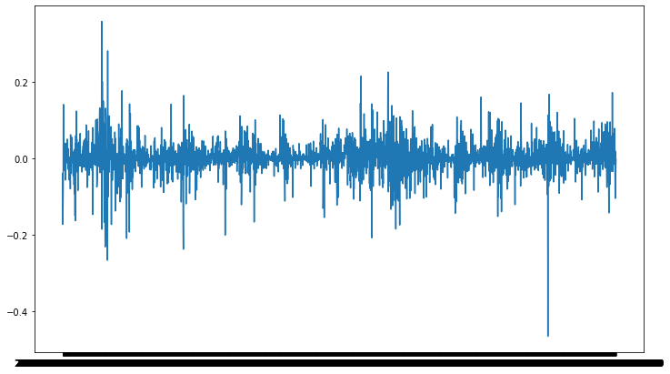
As seen in the Log returns curve, the values oscillate around the zero mean value, thus indicating stationarity.
x = required_data[[‘Close’,’Log returns’]].values #The requires data fields are the Close price and Log returns
Next stop, data normalization. Normalization helps to narrow values to a range 0?—?1 so as to annul the effect of data points constituting high standard deviation. This means that in a situation where later values are significantly higher than earlier values (as with Bitcoin), normalization will help to reduce the effect of higher values on the overall prediction.
We then import the relevant libraries:
from sklearn.preprocessing import MinMaxScaler
from sklearn.preprocessing import StandardScaler
scaler = MinMaxScaler(feature_range=(0,1)).fit(x) # we pass the relevant data to the MinMax scaler
x_scaled = scaler.transform(x)
For the training the model outputs, we specify only the closing price as that is what we want to predict in the end.
y = [x[0] for x in x_scaled] #Using the slice notation to select the Close price column
Now we want to allocate 80% of the data as training set and 20% as test set, an so we specify a split point
split_point = int(len(x_scaled)*0.8) # This amounts to 2288
Creating the training and testing sequence:
x_train = x_scaled[:split_point]
x_test = x_scaled[split_point:]
y_train = y[:split_point]
y_test = y[split_point:]
We then try to verify that the datasets have the right dimensions:
assert len(x_train) == len(y_train)
assert len(x_test) == len(y_test)
Now we label the model:
time_step = 3 # the time step for the LSTM model
xtrain = []
ytrain = []
xtest = []
ytest = []
for i in range(time_step,len(x_train)):
xtrain.append(x_train[i-time_step:i,:x_train.shape[1]]) # we want to use the last 3 days’ data to predict the next day
ytrain.append(y_train[i])
for i in range(time_step, len(y_test)):
xtest.append(x_test[i-time_step:i,:x_test.shape[1]])
ytest.append(y_test[i])
The input structure of the LSTM architecture:
- Number of observations
- time steps
- number of Features per step
np.array(xtrain).shape #We check for the shape of out train data
result: (2285, 3, 2)
We then create arrays for the training set and test set in line with the input structure of the LSTM architecture:
xtrain, ytrain = np.array(xtrain), np.array(ytrain)
xtrain = np.reshape(xtrain,(xtrain.shape[0],xtrain.shape[1],xtrain.shape[2]))
xtest, ytest = np.array(xtest), np.array(ytest)
xtest = np.reshape(xtest,(xtest.shape[0],xtest.shape[1],xtest.shape[2]))
Now we import the requisite libraries for training the model:
from keras.models import Sequential
from keras.layers import LSTM, Dense
# the input shape comprises the time step and the number of obsevations
model = Sequential()
model.add(LSTM(4,input_shape=(xtrain.shape[1],xtrain.shape[2])))
model.add(Dense(1))
model.compile(loss=”mean_squared_error”,optimizer=’adam’)
model.fit(
xtrain,ytrain,epochs=100,validation_data=(xtest,ytest),batch_size=16,verbose=1)
After successfully training the model, we then test it:
# Prediction phase
train_predict = model.predict(xtrain)
test_predict = model.predict(xtest)
Next stop, we inverse transform our data to obtain the values in the right scale (since it was initially normalized)
# Here we are concatenating with an array of zeros since we know that our scaler requires a 2D input
train_predict = np.c_[train_predict,np.zeros(train_predict.shape)]
test_predict = np.c_[test_predict,np.zeros(test_predict.shape)]
print(train_predict[:5])
print(test_predict[:5])
result:
[128.9825366589186, 128.791668230779, 250.81547078082818, 145.12735086347638, 107.12783401435135] [11970.829458753662, 11754.452530331122, 11848.608578931486, 11352.281297994365, 11475.612062204065]
Now we want to know how our model has fared, and so we check our training and test scores:
from sklearn.metrics import mean_squared_error
train_score = mean_squared_error([x[0][0] for x in xtrain],train_predict, squared=False)
print(‘Train score: {}’.format(train_score))
test_score = mean_squared_error([x[0][0] for x in xtest],test_predict,squared=False)
print(‘Test score: {}’.format(test_score))
result:
Train score: 4420.036011547039 Test score: 13957.621757708266
Now we want to do a comparative plot of the original price as against the LSTM model’s prediction:
original_btc_price = [y[0] for y in x[split_point:]] # generating the original btc price sequence
original_btc_price[:5]
plt.figure(figsize=(20,10))
plt.plot(original_stock_price,color=’green’,label=’Original bitcoin price’)
plt.plot(test_predict,color=’red’,label=’Predicted Bitcoin price’)
plt.title(‘Bitcoin price prediction using LSTM’)
plt.xlabel(‘Daily timeframe’)
plt.ylabel(‘Price’)
plt.legend()
plt.show()
End Note:
We can see that while the predicted values are not exactly the same as the original values, the model predicted the overall direction reasonably well. I believe that this model can be combined with other models (like the Autoregressive Integrated Moving Average model) to proffer better insights as to the overall market sentiments.
NB: This article does not constitute a financial advice as it is solely intended to demystify the financial markets (with Bitcoin as a case study), and show how machine learning can be leveraged-on to investigate different financial assets. Cheers!
Github link here.
References
- Kaggle
- Tradingview
- Medium
- Researchgate